Interactive Computing in Scala with Jupyter and almond

The Scala REPL is a great tool for trying out code interactively. It lets you write expressions in a terminal window, and immediately prints the return value as well as any outputs to the console. Whether you’re learning the language, exploring an API, or sketching out a new idea, the immediate feedback after evaluating an expression is a great enabler for hands-on learning and rapid prototyping.

The easiest way to get started is the default REPL because it’s part of the Scala distribution and is also available in any SBT project as the console command. The default REPL lacks many convenience features though.

Ammonite

Ammonite is a modern REPL implementation created by Li Haoyi. It comes with many features that make working in the REPL more convenient. Probably the most important one is dynamic maven dependency loading in the REPL itself (through Coursier), which allows you to import and immediately use almost any published Scala or Java library. It also has many others convenience features, such as * multi line editing support * better syntax highlighting. i.e. inputs are highlighted as you type * much better autocompletion * pretty printed, nicely formatted outputs * undo/redo, session handling and more

If you know Python, Ammonite (roughly) is to the default Scala REPL what the IPython shell is to the default Python shell. Parts of Ammonite are also used in the default dotty REPL, which means they will be available in Scala 3.

While Ammonite has many improvements compared to the default REPL, the basic execution model is still the same. You enter an expression (or multiple expressions in a block). You press enter to have it evaluated to immediately see the output below your input. You then repeat with a new expression or by refining the previous one and executing it again. As a result, your inputs are interleaved with the computed output values.

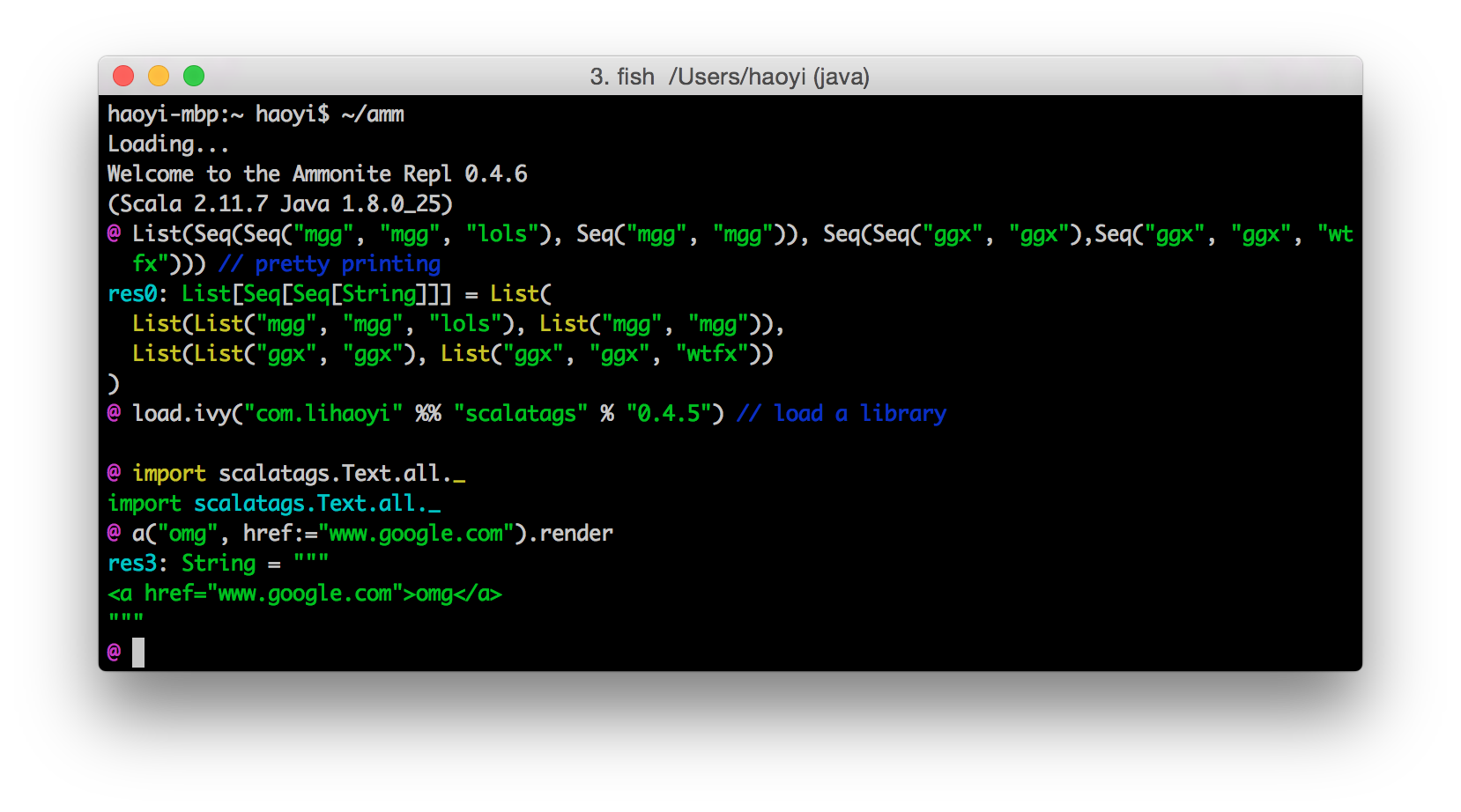The Ammonite REPL (Source: ammonite.io)

This model of interaction helps you to iterate fast due to the immediate feedback, but it also has some drawbacks: * Seeing multiple inputs at once can be hard, because they are interleaved with their outputs, especially if the outputs are long. * It also makes it harder to copy multiple consecutive inputs into an editor. * Finding and changing older inputs often means scrolling back or searching the history because they are far away or in the console window completely gone due to newer outputs. * Selectively replaying multiple expressions after changes in an earlier input or after a REPL restart can be tedious.

You can show the history of inputs using :history in the default REPL or repl.history in Ammonite. While the history can be helpful, it is often cluttered with refinement attempts, which you still need to filter out.

An interesting REPL variant that addresses some of these issues are worksheets.

Worksheets

From the Dotty documentation:

A worksheet is a Scala file that is evaluated on save, and the result of each expression is shown in a column to the right of your program. Worksheets are like a REPL session on steroids, and enjoy 1st class editor support: completion, hyperlinking, interactive errors-as-you-type, etc.

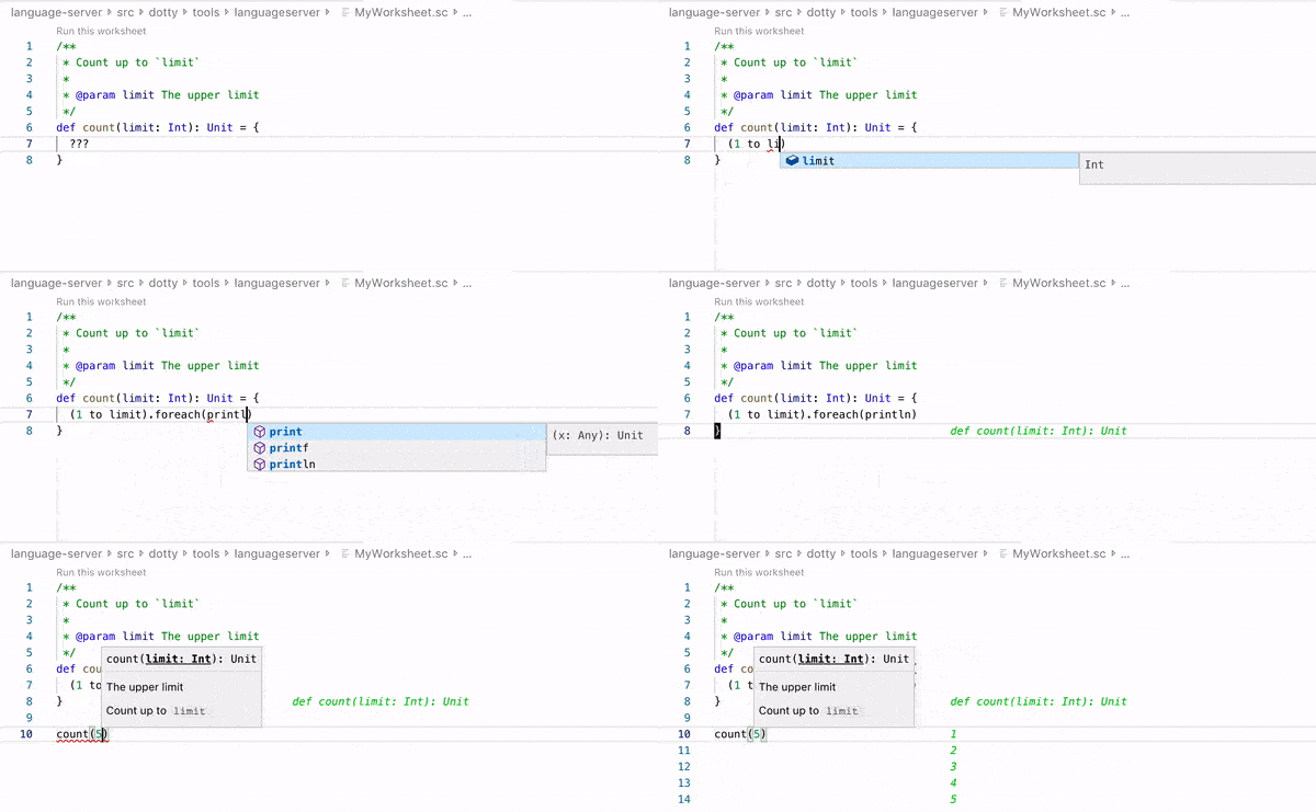
Worksheet example in Dotty IDE / Visual Studio Code. (source: Dotty documentation)

Let’s go through this definition to explain how worksheets differ from the REPL:

First of all, worksheets are files. That means we can put them under version control and share them with others more easily.

Second, we enter our expressions into an editor window. In most cases, the input editor is on the left while the output is shown to the right. This layout makes it easier to see multiple expressions at once, because they are not interleaved with their outputs. It also makes it easier to write multi line expressions and to edit expressions.

Third, a worksheet is evaluated on save. More specifically, all expressions are recomputed every time we save the worksheet. The advantage of this behaviour is that it’s easy to change an earlier expression because all dependent values are automatically recomputed. The drawback is that you lose control over which expressions are evaluated so it’s not very well suited for things that take longer than a few seconds like loading large datasets or running complex computations.

The fourth point about editor support is mostly IDE dependent. Dotty IDE worksheet support looks very nice, but most of us are still stuck with Scala 2. I’ve tried IntelliJ worksheets a few times but they didn’t work very well for me. Eclipse based Scala IDE had good worksheet support last time I tried it but isn’t widely used for other reasons. There’s also an online worksheet variant called Scastie that only requires a browser and makes it very easy to share worksheets online.

So worksheets solve some of the issues of REPLs mentioned above. Their layout and their execution model makes multiple expressions easier to read and to change, even if their outputs are shown. However, the execution model also introduces new issues.

So the natural question that follows is: Could we combine the advantages of REPL and worksheets somehow? Interestingly, there is a technology that does have most of the advantages of both (and more): Jupyter notebooks.

Jupyter Notebooks

Jupyter notebooks are interactive, web based documents that can contain executable code. Interactive notebooks are nothing new. In science, they’re in use since the 80s and many different flavours exist.

As of today though, Jupyter notebooks are by far the most successful and flexible variant. Some reasons for their success are that they’re open-source, programming language agnostic, provide a modular architecture and a web-based frontend. That’s why we will use Jupyter as an example to explain the basic concepts behind interactive notebooks. In fact, this article itself is written as a Jupyter notebook.

A Jupyter notebook is made of editable input cells. Cells can be of different types. By default, two cell types are available:

Documentation cells, which are written in Markdown and rendered to HTML when we run them, using JavaScript directly in the browser. For instance, this text was written as a Markdown cell, and you see the HTML output.
Code cells, which allow you to write and execute code.

Here’s a simple example of a Scala code cell:

println("Hello notebook!")
val x = 42

Hello notebook!

x: Int = 42

Code cells are executed by so called kernels. A kernel is basically an interpreter process that executes the code of a code cell in the backend. Once you run a code cell, the frontend sends the current cell content to the kernel for processing. The kernel’s output is then sent back to the frontend and written below the code cell. Later cells can access the variable state of previous cells as long as the kernel is still running.

x / 2 + 2

res1: Int = 23

Jupyter Kernels can be implemented in any language as long as they follow the ZeroMQ based Jupyter communication protocol. IPython is the most popular kernel and is included by default. That’s no surprise since Jupyter (Julia, Python, R) is derived from the IPython project. It is a result of separating the language independent part from the IPython kernel to make it work with other languages. Now there are kernels for over 100 programming languages available.

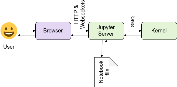
High level overview of the Jupyter components (source: Jupyter documentation)

The Jupyter frontend renders the notebook and lets you interact with it. It provides editing capabilies, lets you create notebooks, execute cells and so on. The default frontend Jupyter classic is made of HTML & JavaScript and runs in the browser. In 2018, a modern, more flexible and modular frontend implementation called JupyterLab was published as “the next-generation web-based user interface for Project Jupyter”.

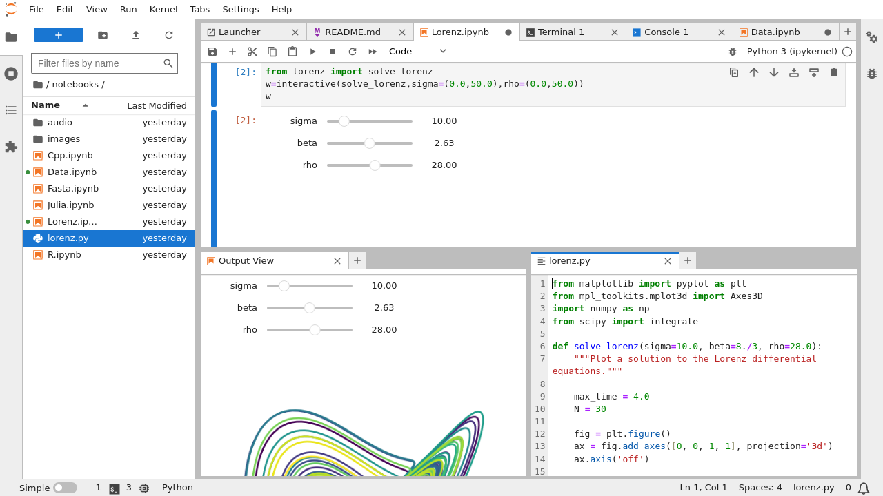
The JupyterLab interface (source: JupyterLab documentation)

The modular architecture of Jupyter allows you to run kernels anywhere: On your laptop, in the cloud, or on a powerful GPU machine for deep learning. The frontend on the other hand even runs on a tablet. You only need a modern web-browser.

There are also desktop frontends with additional features like nteract. A large ecosystem around Jupyter provides various extensions like git integration, specialized widgets etc.

Besides kernel and frontend, a Jupyter installation consists of the language agnostic backend part that manages kernels, notebooks and the communication with the frontend. This component is called the Jupyter server. Notebooks are stored in .ipynb files, encoded in a Json format on the server. The Json based format allows storing cells inputs, outputs and metadata in a structured way. Binary output data is base64encoded. The disadvantage is that the json makes diff and merge harder, compared to line based text formats. You can export notebooks into other formats such as Markdown, Scala (contains only code input cells), or HTML like this article.

Jupyter and Scala

How does support for Jupyter look like in Scala? There’s actually a number of different Scala kernels available. If you look closer though, many of them are somewhat limited in features, have scalability issues or have even been abandoned. Others are focused exclusively on Spark rather than Scala in general and other frameworks.

One reason for that is that almost all existing kernels build on top of the default REPL. Due to its limitations, they customize and extend it to add their own features such as dependency management or framework support. Some kernels also use the Spark Shell which is basically a fork of the Scala REPL customized for Spark support. This all leads to fragmentation, difficulty of reuse and duplication of work, making it harder to create a kernel that is on par with other languages.

For a more detailed discussion about some of the reasons check out this talk at JupyterCon 2017 by Alexandre Archambault:

Scala: Why hasn't an Official Scala Kernel for Jupyter emerged yet?

The almond Scala Kernel

Fortunately, recent developments have changed the situation. We’ve already talked about Ammonite and the improvements it has over the default REPL. Couldn’t we leverage some of Ammonite’s features for a Scala kernel as well? And that’s exactly what almond (formerly called jupyter-scala) by Alexandre Archambault does. By building on top of Ammonite, almond can directly benefit from many of its features.

For instance, dynamic dependency resolution works exactly the same way as in Ammonite:

import $ivy.`org.typelevel::cats-core:1.5.0`
import cats.syntax.semigroup._ // for |+|
import cats.instances.int._    // for Monoid
import cats.instances.option._ // for Monoid

Option(1) |+| Option(2)

import $ivy.$                               
import cats.syntax.semigroup._ // for |+|
import cats.instances.int._    // for Monoid
import cats.instances.option._ // for Monoid
res2_4: Option[Int] = Some(3)

The same is true for syntax highlighting, pretty printing and autocompletion.

Seq.fill(5)(Seq.fill(3)("Foo"))

res3: Seq[Seq[String]] = List(
  List("Foo", "Foo", "Foo"),
  List("Foo", "Foo", "Foo"),
  List("Foo", "Foo", "Foo"),
  List("Foo", "Foo", "Foo"),
  List("Foo", "Foo", "Foo")
)

Building on Ammonite also highlights a more general design principle of almond. It tries to delegate as much functionality as possible to existing components instead of reinventing the wheel. Doing so allows it to stay more lightweight, easier to understand, and to better focus on its core functionality as a kernel. While almond has used a forked version of Ammonite for some time, the changes have been upstreamed and it now includes stock Ammonite. This is unlike other kernels which have often heavily customized and extended the Scala REPL to fit their needs.

almond is not tied to a specific big-data framework like Spark. That doesn’t mean we can’t have framework integrations, quite on the contrary. But the idea is to do bridging and integration in more standardized way instead of having to customize the REPL or the kernel itself. Ideally, the integration is done as a module or a separate library that talks to the kernel via well defined APIs. For interfacing with a Spark cluster for instance, almond relies on ammonite-spark in combination with providing a Jupyter specific Spark module.

Due to its modular design and well defined interfaces, almond even makes it easy to create your own custom kernel. For more info about almond’s features, check out its project website.

almond development (through its creator and main developer) is currently funded by the Scala Center but there’s still a lot to be done, like adding more integrations or improving the code editor experience for Scala. If you’d like to contribute, PRs are very much welcome!

Combining the Advantages of REPLs and Worksheets

Let’s now get back to the question how Jupyter notebooks combine the advantages of REPLs & worksheets. In a sense, you can think of a notebook as a REPL of worksheets (cells).

Each code cell roughly corresponds to a worksheet. You have an editor window to enter your expressions, and once you hit run, all expressions in a cell are evaluated in one go and the outputs are shown below. Since notebooks are files, you can also save them, share them and put them under version control like worksheets. So the behaviour inside a cell is basically worksheet like, except that by default, the output is not on the right hand side but below the cell.

A Jupyter notebook can have as many cells as you like, though, and at the document level it behaves more like a REPL. You enter one or more expressions in a cell, run it, perhaps refine and run again a few times until you’re happy. Then you create a new cell below the current one (which may depend on values from the cell above) and repeat the process. The way you can control which cell will be executed is actually even more flexible. You can, for instance * select any cell and (re-)run it * Run all cells, or all cells above/below the currently selected cell * Insert a new cell anywhere, or delete an existing one * copy and paste cells * easily rearrange cells as you like * merge or split cells

That’s a very powerful toolbox for experimentation. Because you can execute and rearrange cells arbitrarily, sometimes you end up with cells containing expressions which depend on values from cells below. This can be very confusing so you should make sure that your code runs fine when executing your notebook in linear order, especially if you want to share it. There’s a talk called I Don’t Like Notebooks by Joel Grus about those traps and about Jupyter notebooks from a Software Engineering perspective.

Since cells in one notebook share the same kernel and its interpreter variable state, they can depend on values computed by other cells executed earlier. So you could have a cell on top of your notebook that loads a large dataset or runs a complex computation and the results will be cached and available to all cells executed later, as long as the kernel isn’t restarted. In essence, notebooks defuse the main disadvantage of worksheets by combining its execution model with the one of the REPL.

While outputs are shown below a cell by default, interleaving of input and output is between cells, not between single expressions as in The REPL. That means you can always see the code of a cell as a whole. You can also easily clear the output of a cell or of all cells to see all your inputs more clearly. Last but not least can you also export your notebook as a Scala file containing all your code input cells.

Rich, Interactive Computing in your Browser

Another very important reason why Jupyter notebooks are so successful is their web based frontend and how we can interact with it. As we’ve already seen, we can add documentation cells with Markdown formatting including images or other HTML elements. But what makes notebooks really powerful is that the Jupyter API allows us to send rich outputs from the kernel to the frontend.

We can generate generate dynamic web content on the fly in our code, accessing any data source available and send it to the frontend. That way, we can display basically anything the browser supports such as tables, images, charts etc. straight from our code. We can even send JavaScript from the kernel that will be executed in our frontend. And that JavaScript can communicate with the kernel through the Jupyter API i.e. for interactive input widgets.

This powerful idea is best illustrated with a few examples:

import almond.interpreter.api.DisplayData

display(
  DisplayData(
    Map(
      "text/html" -> "Some <b>HTML</b>")))

Some HTML

import almond.interpreter.api.DisplayData

The kernel API provides a display method that takes expects our content, together with its mime-type. We can also send multiple representations of the data we want to display (keyed by mime-type), and the frontend will pick and show the most specific one it supports:

display(
  DisplayData(
    Map(
      "text/plain" -> "Some text",
      "text/html" -> "Some <b>HTML</b>")))

Some HTML

almond provides and automatically imports some convenience helper methods for common mime-types in almond.api.helpers.Display:

html("Some <b>HTML</b>")

Some HTML

res6: almond.api.helpers.Display = text/html #e207fdff-f77e-464b-acb7-3c2a882d6292

You can also register a Displayer for any type via JVM Repr, a project for “standardizing object representation and inspection across JVM kernels (Scala, Clojure, Groovy, …)”.

Let’s see how a list of people is displayed by default:

case class Person(name: String, age: Int)
case class People(people: Seq[Person])

val people = People(
  Seq(
    Person("alice", 29),
    Person("bob", 23),
    Person("charlie", 34)
  )
)

defined class Person
defined class People
people: People = People(
  List(Person("alice", 29), Person("bob", 23), Person("charlie", 34))
)

Now let’s add a displayer for People and see how it is displayed:

import $ivy.`com.lihaoyi::scalatags:0.6.7`

import jupyter.Displayer, jupyter.Displayers
import scala.collection.JavaConverters._

// Note that as of now this approach doesn't seem to work with parameterized types like Seq[Person]
// which is probably due to type erasure.
Displayers.register(classOf[People], (people: People) => {
  import scalatags.Text.all._
  Map(
    "text/html" -> {
      table(cls:="table")(
        tr(th("Name"), th("Age")),
        for (Person(name, age) <- people.people) yield tr(
          td(name),
          td(age)
        )
      ).render
    }
  ).asJava
})

people

Name	Age
alice	29
bob	23
charlie	34

import $ivy.$                             
import jupyter.Displayer, jupyter.Displayers
import scala.collection.JavaConverters._
// Note that as of now this approach doesn't seem to work with parameterized types like Seq[Person]
// which is probably due to type erasure.

Pretty neat huh?

The idea is that library authors can provide Displayers for types i.e. for a Spark DataFrame and once you have it imported it you will get a nicely formatted representation of your data.

There are also helpers for images.

Image.fromUrl("https://scala-lang.org/resources/img/frontpage/scala-spiral.png", width=Some("50"))

res9: almond.api.helpers.Display = image/png #422d85e7-fa35-467d-be50-ebe246d13a69

Let’s see a more advanced example. We can easily plot nice, interactive charts directly in our notebook using Plotly and the plotly-scala bindings.

import $ivy.`org.plotly-scala::plotly-almond:0.5.4`
import plotly._, plotly.element._, plotly.layout._, plotly.Almond._
{{  
  val trace1 = Scatter(
    Seq(1, 2, 3, 4),
    Seq(0, 2, 3, 5),
    fill = Fill.ToZeroY
  )

  val trace2 = Scatter(
    Seq(1, 2, 3, 4),
    Seq(3, 5, 1, 7),
    fill = Fill.ToNextY
  )

  val data = Seq(trace1, trace2)

  plot(data)
}}

import $ivy.$                                      
import plotly._, plotly.element._, plotly.layout._, plotly.Almond._
res10_2: String = "plot-25d7d03f-0ef2-42ed-92a7-564179c52cc0"

Here we use the ability to send JavaScript to generate inject the plotly widget into our frontend. Newer frontends like JupyterLab and nteract are more restrictive about JavaScript execution for security reasons. That’s why plotly-scala also sends a json representation of our plot which is then rendered by nteract or the JupyterLab Plotly extension.

Communicating results

The ability to generate and display rich (and possibly interactive) outputs is an invaluable tool for interactive data exploration and analysis, machine learning, and science experiments. That’s why interactive notebooks have recently been named the third most important tool for data scientists. Being able to show your code side-by-side with documentation, rich outputs and visualizations can be a very effective way to communicate results.

Teaching and Learning

Notebooks are also an interesting tool for teaching and learning. They can help you to create executable tutorials, docs and examples. For instance, I’ve recently converted the Scala Tour into a set of Jupyter notebooks you can run on Binder.

Visualize your data structures

Or how about experimenting with a nice inline visualization of your data structures using the amazing reftree library?

import $ivy.`io.github.stanch::reftree:1.3.0`

{{
  import reftree.render._, reftree.diagram._
  import reftree.contrib.SimplifiedInstances.string
  val renderer = Renderer(renderingOptions = RenderingOptions(density = 75))
    
  case class Person(name: String, age: Int)
  val people = List(
    Person("Alice", 29),
    Person("Bob", 23),
    Person("Charlie", 34)
  )

  renderer.render("example", Diagram.sourceCodeCaption(people))
}}
Image.fromFile("example.png")

Downloading https://repo1.maven.org/maven2/xml-apis/xml-apis-ext/1.3.04/xml-apis-ext-1.3.04-sources.jar.sha1
Downloading https://repo1.maven.org/maven2/xml-apis/xml-apis-ext/1.3.04/xml-apis-ext-1.3.04-sources.jar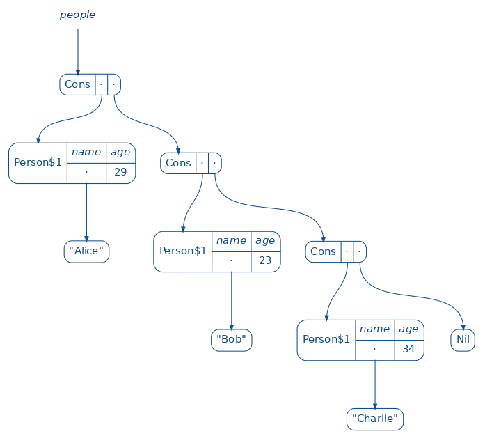

import $ivy.$                                
res11_2: almond.api.helpers.Display = image/png #c6b66980-c2ad-48e7-9a40-2ee06df0a5ce

Conclusion

I hope that I could convince you that Jupyter notebooks are a powerful and incredibly flexible tool for interactive computing. As we’ve seen, they combine many strengths of the REPL and worksheets, while also adding unique new features. Their web-based interface, interleaving code with documentation, and the ability to send rich outputs from your code to the frontend give you a wealth of possibilies for things like prototyping, data visualization, communication of results, and teaching.

The almond kernel makes that power available for Scala, including all the niceties of Ammonite. Even though it still needs some more integrations and documentation, it’s already quite usable and fun to work with.

To see more examples of what’s possible with Jupyter and almond, check out the examples repo. It consists of a growing collection of Jupyter notebooks, each containing executable Scala code. You can run all these notebooks in your browser without any local setup, using Binder.

If you have any questions or feedback, don’t hesitate to leave a comment, or ping me on Twitter @soebrunk.